Pontryagin’s Maximum Principle, Intuitively

Optimus Prime - leader of the Autobots

Introduction

Let’s say I have a robot. Or a 3D printed Relativity Federal rocket. Or let’s say we have a transformer (the Optimus Prime kind). These are all things that we can model with dynamical systems: mathematical models that allow us to describe how a system’s state evolves over time based on constraints (or fixed rules). Although modeling Optimus Prime might be a bit more complex since he he’s got a mind of his own. You get the point.

In optimal control, we want to find the best way to steer a dynamical system over time, in order to achieve some goal, or minimize cost while respecting the constraints. While machine learning methods have become increasingly powerful in improving such complex modeling and data analysis, we would rather rely on provable stability and optimality guarantees, which ML often lacks. We’ll look at something called Pontryagin’s Maximum Principle, which is a method used to find the best possible control for taking a dynamical system from one state to another.

A Control Problem

Let’s look at this method from the context of a control problem. In optimal control, we usually start with a function that defines the system’s initial condition. We can do this with the given initial value problem:

\[\dot{x}(t) = f(x(t), u(t))\] \[x(0) = x_0\]

$x$ is the state
$u$ is the control
$f$ is a known function representing the dynamics

What’s the goal? In optimal control we want to find a control function $u^*$ such that the trajectory $(x^*(t), u^*(t))$ across the time interval minimizes some performance measure which we can call $C(x,u)$. Again, this can be minimizing cost or deviation from a pre-determined goal.

\[C(x,u) = q_T(x(t_f), t_f)+ \int_0^{t_f} g(x(t), u(t))\,dt\]

$q_T$ is the terminal cost (terminal meaning until completion)
$g$ is the running cost
$t_f$ is the terminal time

Surprise! We end up with a constrained optimization problem:

\[\begin{aligned} \min_{x,u} \quad & C(x,u) \\ \text{s.t.} \quad & \dot{x}(t) = f(x(t), u(t)) \end{aligned}\]

Solving the Optimization Problem

Let’s pause briefly here. At this point, we’re trying to solve a problem that looks like optimization, but is actually different. We are optimizing over functions $x(t)$ and $u(t)$, not vectors. This means our constraint $\dot{x}(t)$ must hold at every time $t$. This is pretty difficult — it’s infinite-dimensional.

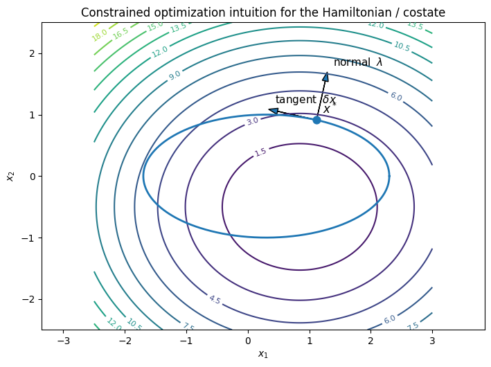
In finite dimensions, we would minimize a function subject to constraints via Lagrange multipliers. Now we introduce something called the Hamiltonian, which essentially does the same thing, but applied continuously in time.

We introduce a time-varying Lagrange multiplier $\lambda(t)$ (which is often called the adjoint variable) and add a penalty term to the cost functional:

\[\int_0^{t_f} \lambda(t)^T \big(f(x(t), u(t)) - \dot{x}(t)\big)\,dt\]

Essentially we want to penalize violations of the constraints using multipliers — which makes sense.

Let’s define the Hamiltonian:

\[H(x,u,\lambda) = g(x,u) + \lambda^T f(x,u)\]

Our new cost objective is then:

\[C(x,u) = q_T(x(t_f), t_f) + \int_0^{t_f} \big(H(x,u,\lambda) - \lambda^T \dot{x}\big)\,dt\]

Optimal control as constrained optimization. The system dynamics restrict trajectories to a feasible manifold. At an optimal trajectory, any feasible variation lies tangent to this manifold. The costate $ \lambda(t) $ arises as a multiplier orthogonal to feasible directions, enforcing stationarity of the cost under the dynamics constraint.

What Does This Mean?

Conceptually, the Hamiltonian bundles together immediate cost and how the current state influences the future. This is actually analogous to how (Q)-functions are defined in traditional reinforcement learning!

The costate (\lambda(t)) basically tells us how valuable it is to change from the state (x(t)) currently. From here, we can apply calculus of variations, which leads to Pontryagin’s Maximum Principle, giving us three coupled conditions on state dynamics, costate dynamics, and the optimal control condition (u^*(t)).

The Big Picture

The Hamiltonian is the continuous-time analogue of a Lagrangian, and it encodes both the immediate cost and future consequences. This enables optimal control to be solved via first-order necessary conditions.

In other words, it converts a global, constrained problem into a local decision rule governed by first-order conditions.